Inclined Shock Tracking
An advanced application of the Shock Tracking Library involves estimating the oblique shock angle. It is sometimes crucial to verify the inflow conditions and assess the unsteady behavior, such as changes in the inclination and oscillation domain. In this tutorial, the first leading edge shock from 100 schlieren images, is tracked as follows:
Run the following piece of code:
from ShockOscillationAnalysis import InclinedShockTracking as IncTrac

if __name__ == '__main__':
    # Define the snapshots path with glob[note the extention of imported files]
    imgPath = r'test_files\raw_images\*.png'

    # iniate the inclined shock tracking module
    IncTrac = IncTrac()

    # use ShockTracking function
    IncTrac.ShockPointsTracking(imgPath,
                                scale_pixels = False,
                                tracking_V_range = [575, 200], # as not scaled tracking reference values in pixels
                                nPnts = 9,                     # number of slices
                                inclination_info = 110,        # width of each slice
                                preview = True,                # to preview the final setup before proceeding
                                slice_thickness = 4,           # number of vertical pixels to be be averaged for each slice
                                points_opacity = 0.5,          # displayed tracked points transparency
                                avg_preview_mode = 'avg_ang',  # to display the estimated shock angle for each snapshot
                                avg_show_txt = True,           # to display the estimated shock angle value
                                avg_txt_Yloc = 650,            # y-location of the estimated angle value in pixels
                                avg_txt_size = 30,             # font size of estimated angle value in pt
                                osc_boundary = True,           # to display the oscilation domain
                                )
The spacified
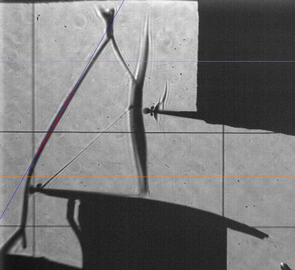
tracking_V_rangeis reviewed, and the estimated shock line is asked: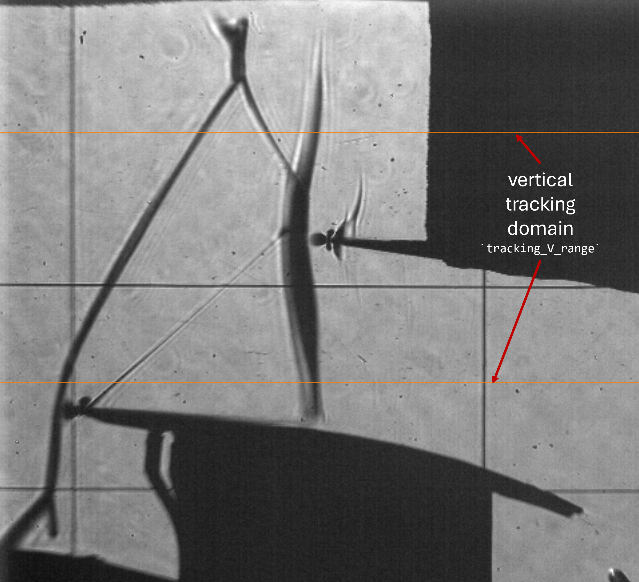
Press the left mouse button and drag to draw a line. Two lines will appear: the bold red line represents the start and end mouse locations, and the blue line represents the full line. Left-click again to confirm flowed by any keyboard key to close the preview window or right-click to remove the line and try again.
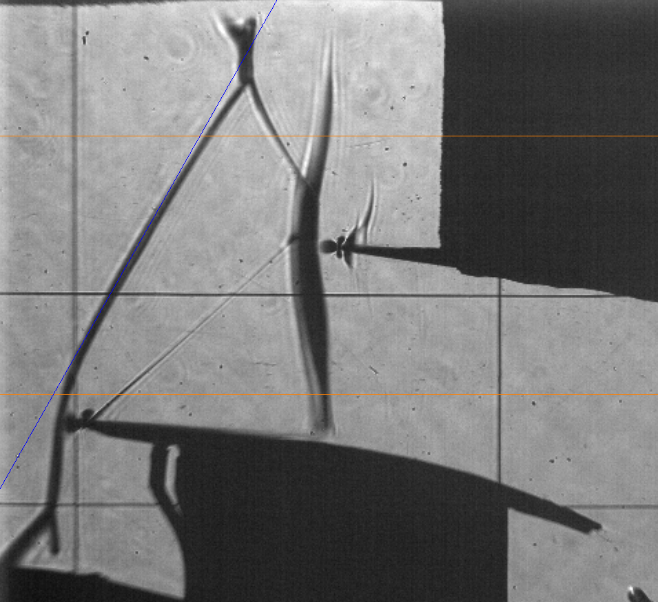
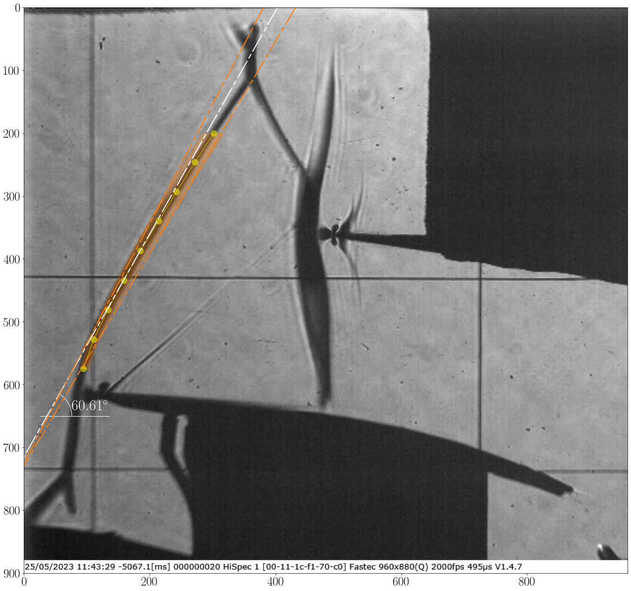
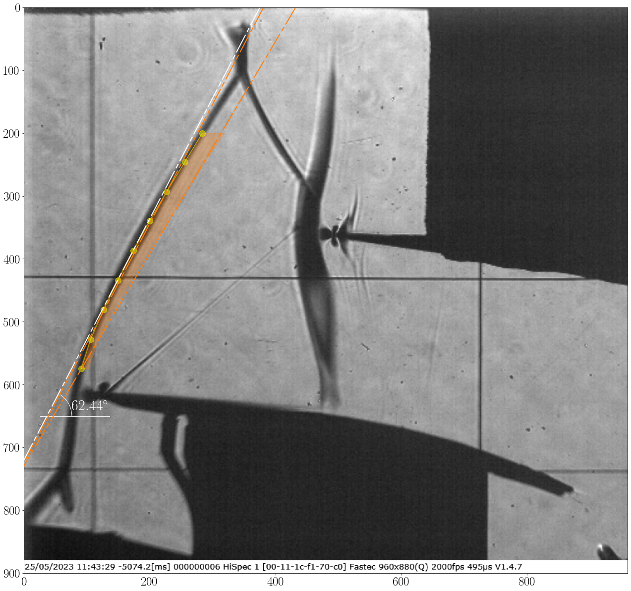
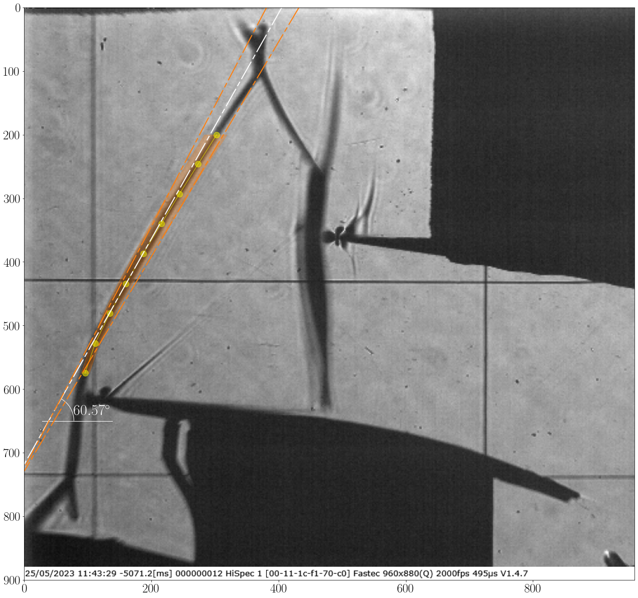
The software will track the shock and show results as follow:
Img Shape is: (900, 960, 3)
Screen resolution: 1920, 1080
Vertical range of tracking points is:
    - In pixels from 200px to 575px
Registered line: ((415, 0), (0, 726), -1.7477477477477477, 726.0270270270271)
Shock inclination test and setup ... ✓
Importing 100 images...
[=================== ] 99%
Shock tracking started ... ✓
Angle range variation: [56.82, 61.46],  σ = 0.94
Average shock loc.: 227.08±0.00 px
Average shock angle: 58.94±0.00 deg
Plotting tracked data ...
info.: For memory reasons, only 20 images will be displayed.
note: this will not be applied on images storing
[====================] 100%
Processing time: 1 Sec
(array([58.93693154,  0.        ,  0.        ,  0.        ,  0.94152004]), array([227.07783223,   0.        ,  23.87470901]))
And the 20 images are displayed, among of them