Mach number estimation

As an application of the Shock Tracking Library the estimation of the local Mach number from Mach waves as well as other vital flow properties such as pressure and temperature, within intricate shock structures. In such scenarios, the presence of pressure taps may obstruct the visibility of the shock system, requiring the utilization of pressure tubes, wires, or another system that may partially block the test section window. Nonetheless, with a thorough understanding of the flow direction, the Mach number can still be accurately determined using the following formula:

\[M_{1} = \frac{1}{\sin \mu}\]

Where $M1$ represents the upstream Mach number, and $\mu$ denotes the angle of the Mach wave with respect to the upstream flow direction. The tracking algorithm operates on a userdefined number of slices within a specified vertical boundary. Additionally, the flow direction can be evaluated using LDA measurements upstream as in this example of the Mach line or through CFD simulation data, which is then interpolated at the tracking locations.

Run the following code:

import numpy as np
from ShockOscillationAnalysis import InclinedShockTracking as IncTrac

if __name__ == '__main__':
    # Define the snapshots path with glob[note the extention of imported files]
    imgPath = r'test_files\raw_images\*.png'

    # Define the velocity vectors as Vx and Vy with the vertical coordinates y
    inflow_path = r'test_files\upstream_Mwave_vel.csv'
    Vxy = np.genfromtxt(inflow_path, delimiter=',', skip_header = 1)

    # iniate the inclined shock tracking module
    IncTrac = IncTrac(D = 80) # D is the reference true length in this case is 80mm

    # use ShockTracking function
    IncTrac.ShockPointsTracking(imgPath,
                                scale_pixels = True,
                                tracking_V_range = [5, 13],  # as scaled tracking reference values in mm
                                nPnts = 3,                     # number of slices
                                inclination_info = 50,         # width of each slice
                                points_opacity = 0.5,          # displayed tracked points transparency
                                avg_preview_mode = 'avg_all',  # to display the estimated shock angle for each snapshot
                                avg_txt_Yloc = 650,            # y-location of the estimated angle value in pixels
                                avg_txt_size = 30,             # font size of estimated angle value in pt
                                flow_Vxy = Vxy,                # inflow velocity vectors [y, Vx, Vy]
                                angle_interp_kind = 'linear',  # inflow data interpolation to match slice points
                                preview_angle_interpolation = True, # to plot interpolation values for review
                                Mach_ang_mode ='Mach_num',     # to show the Mach number values
                                M1_color = 'yellow',           # the displayed Mach number values color
                                M1_txt_size = 18,              # the Mach number values font size in pt
                                arc_dia = 50,                  # the flow angle arc diameter
                                )

Define the scalling lines. Press the left mouse button and drag to draw a line. Two lines will appear: the bold red line represents the start and end mouse locations, and the green line represents the full line. Left-click again to confirm flowed by any keyboard key to close the preview window or right-click to remove the line and try again.

$_static\img\T2\T2-1c.png$

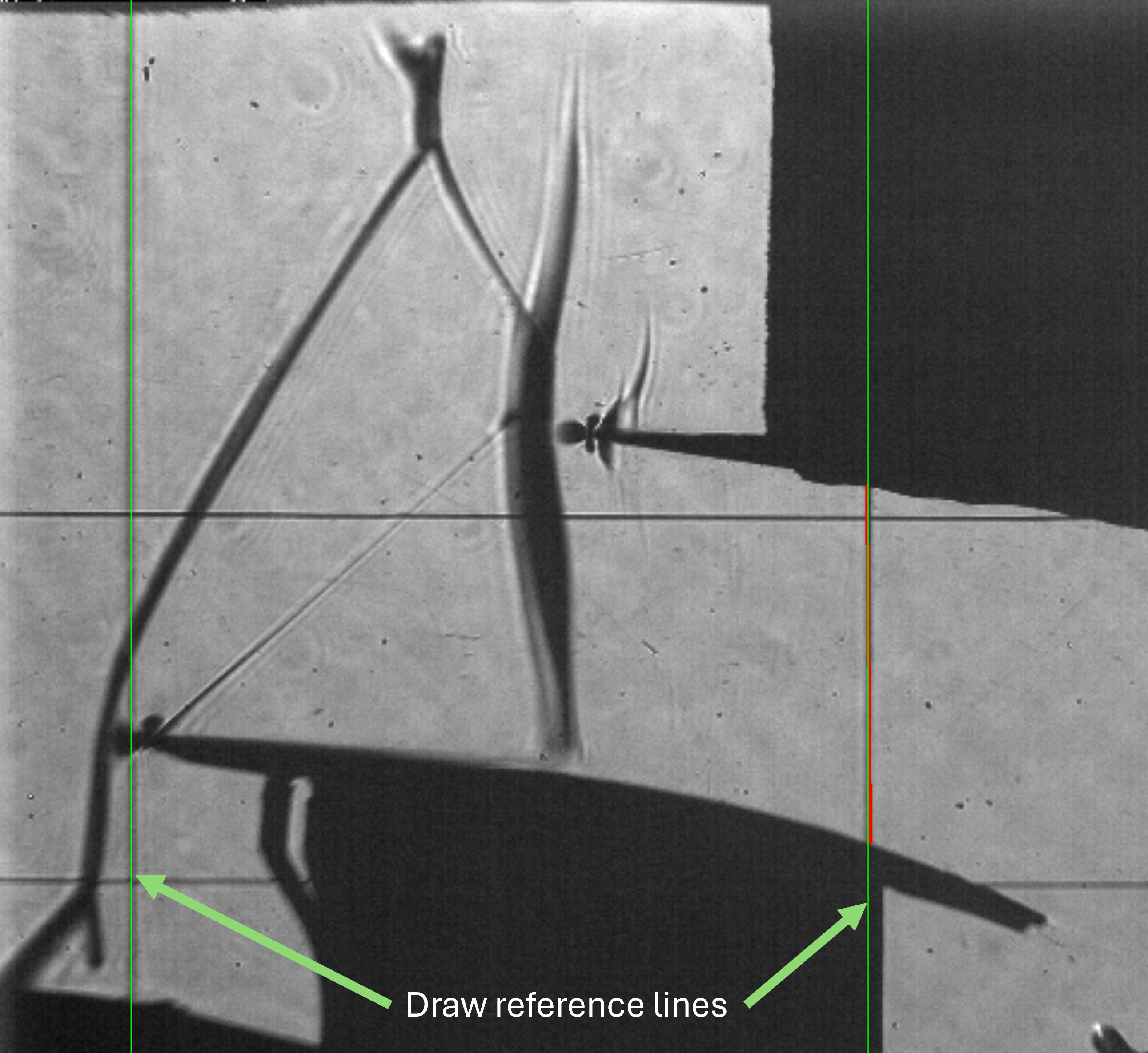
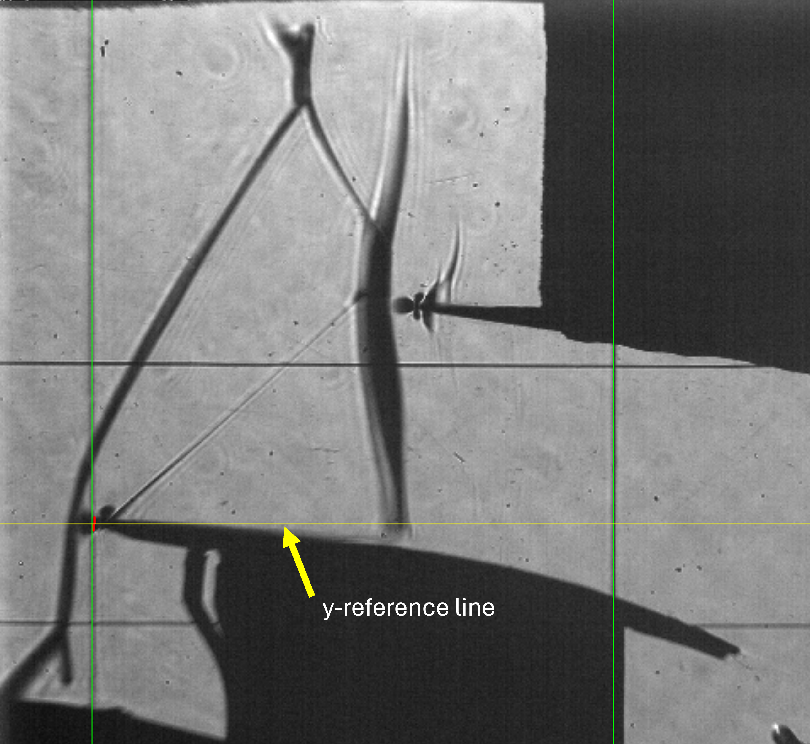
Repeat the drawing process to define y-Reference line (the yellow line in this case the leading of the lower profile)

$_static\img\T2\T2-2c.png$

Important

The vertical lines of scaling and the horsintol line of y-reference are defined as the middle point of start and end of the drawn line.

The spacified tracking_V_range is reviewed, and the estimated shock line is asked, Repeat the drawing process defining the Mach wave: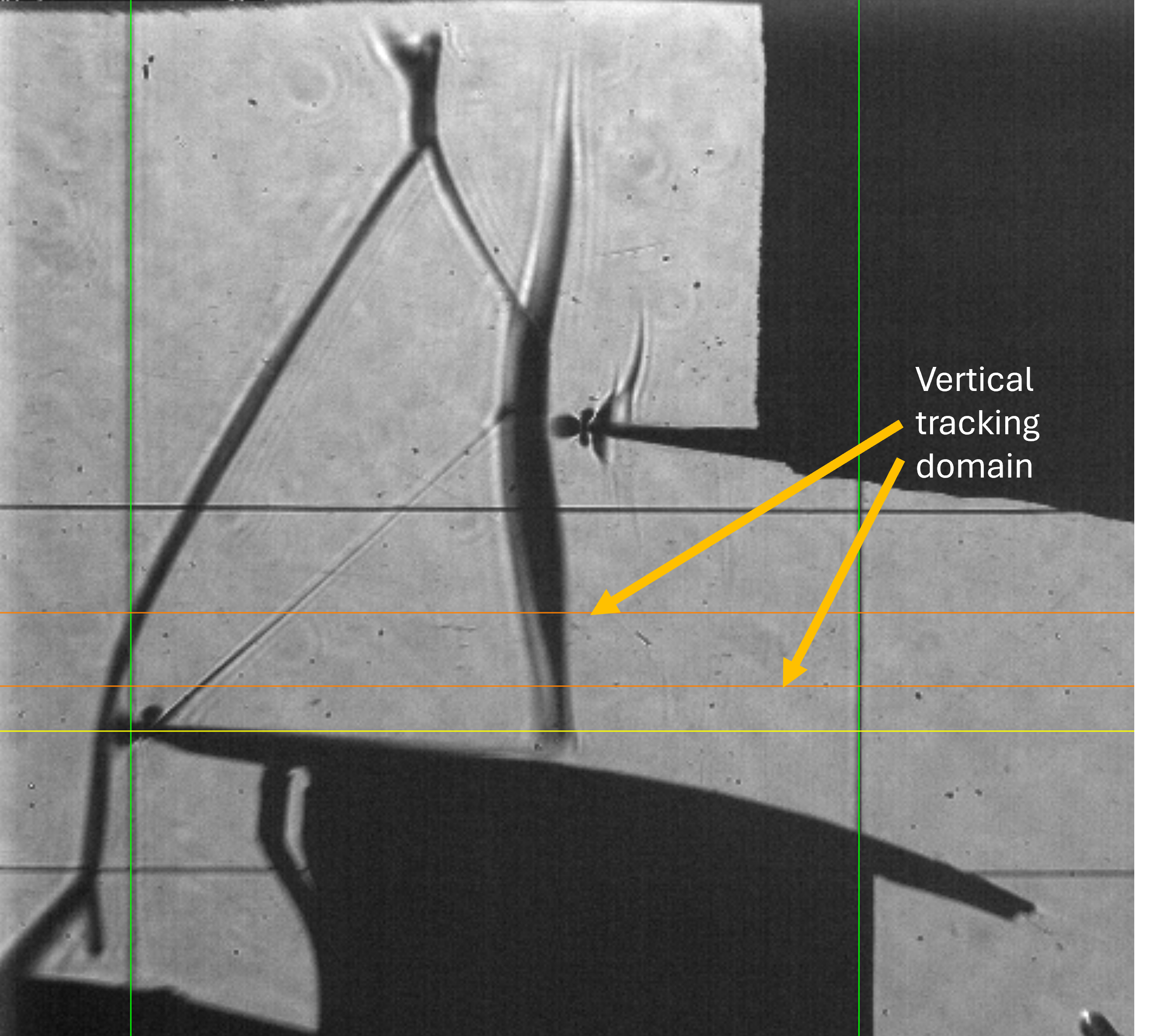

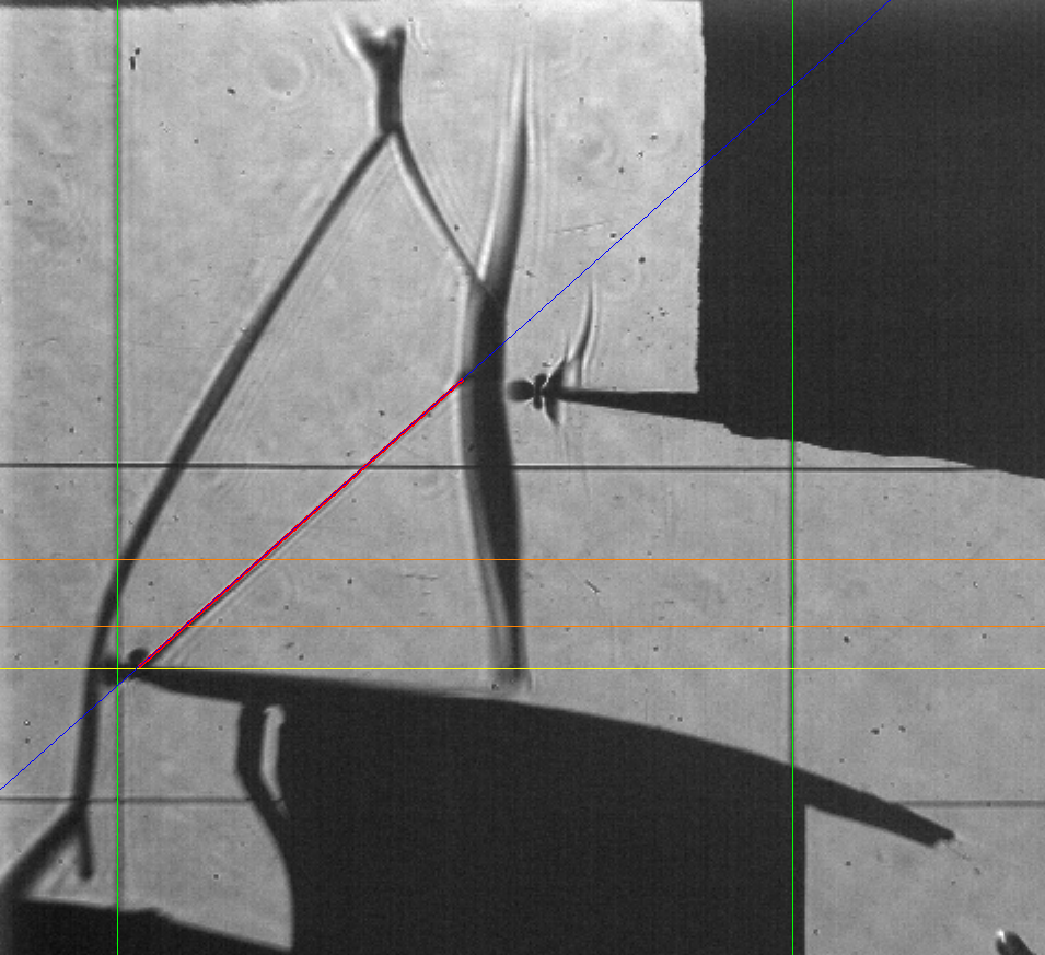
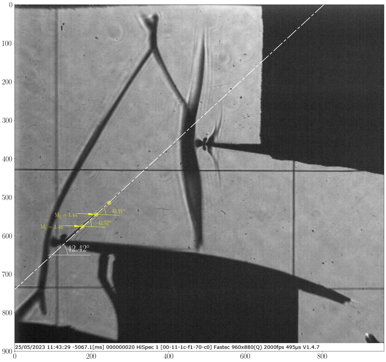
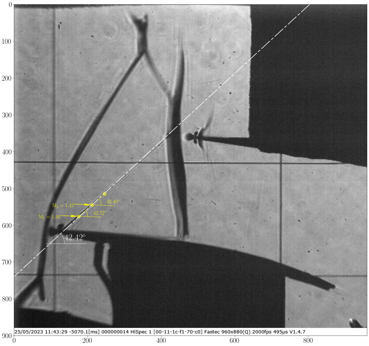
$_static\img\T2\T2-3c.png$ $_static\img\T2\T2-4.png$

The software will track the shock and show results as follow:

Img Shape is: (900, 960, 3)
Registered line: 726
Registered line: 110
Image scale: 0.12987012987012986 mm/px
Registered line: 616
Screen resolution: 1920, 1080
Vertical range of tracking points is:
    - In (mm)s from 5.00mm to 13.00mm
    - In pixels from 516px to 578px
Registered line: ((871, 0), (0, 717), -0.8235294117647058, 717.8823529411765)
Shock inclination test and setup ... ✓
Importing 100 images...
[=================== ] 99%
Warning: Number of points is not sufficient for RANSAC!; Normal least square will be performed.
Shock tracking started ... ✓
Angle range variation: [39.77, 50.29],  σ = 3.23
Average shock loc.: 208.15±0.00 px
Average shock angle: 42.36±0.00 deg
Plotting tracked data ...
info.: For memory reasons, only 20 images will be displayed.
note: this will not be applied on images storing
[====================] 100%
Processing time: 1 Sec

And the 20 images are displayed, among of them

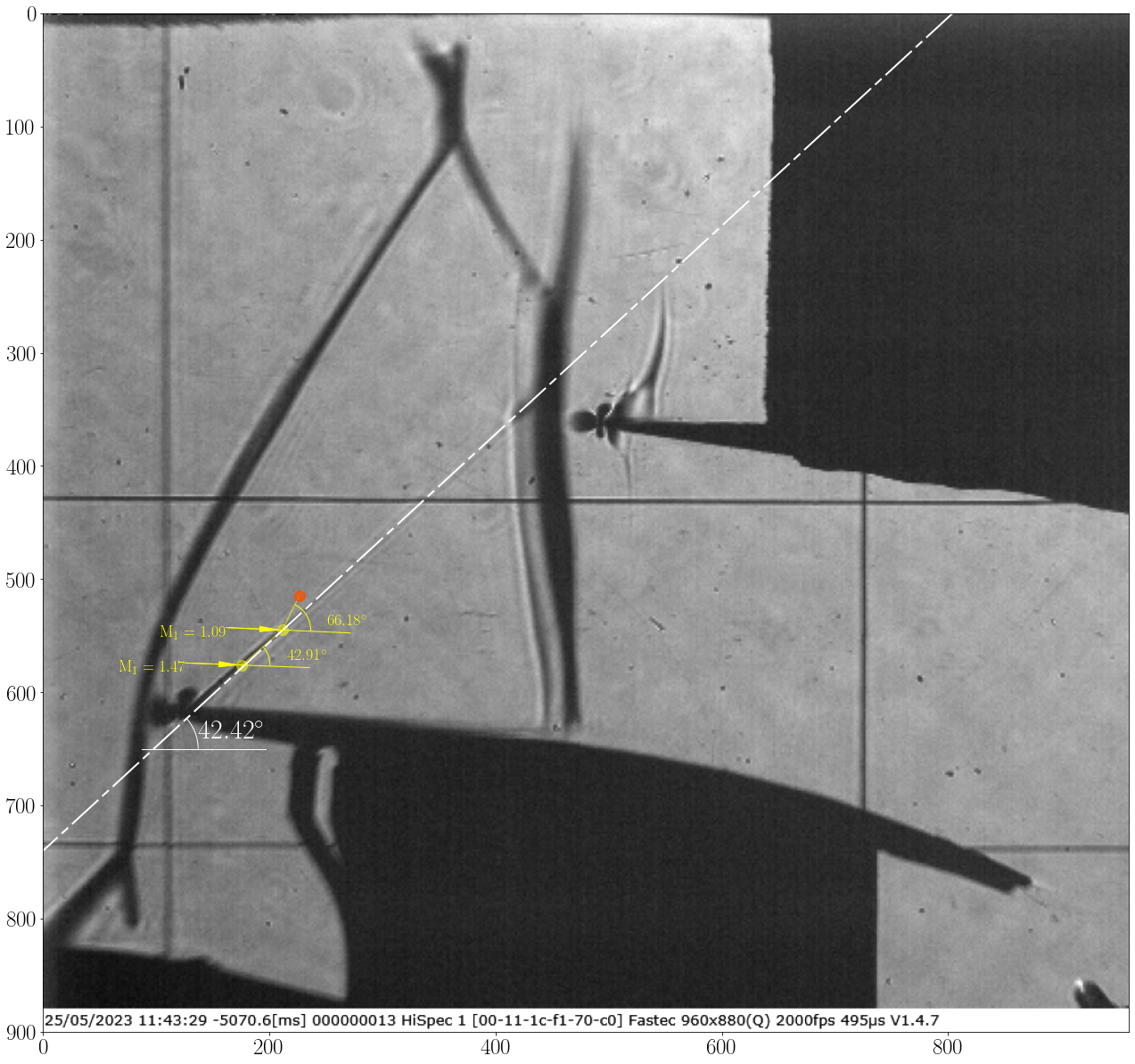
$_static\img\T2\T2-5.png$ $_static\img\T2\T2-6.png$ $_static\img\T2\T2-7.png$

Note

In the second image, there is an orange uncertain point, which completely misses the location of the Mach wave due to its weakness in this region.
The orange uncertain point does not always indicate a false shock location, but it suggests the possibility of missing the shock location.