Slice list generation

In this example, the slice list is generated for line scanning process, the methodolgy was detailed in this artical. This data processing phase involves importing and extracting single-pixel slices from a series of images to create a composite image, which will be further processed and analyzed in subsequent stages.

The GenerateSlicesArray function begins by importing random samples for optimal processing. It tracks the shock within the given slice_thickness, and estimates the average shock angle. Based on the estimated shock angle, the images are rotated, cropped, and averaged into a single-pixel slice to enhance the contrast of the shock. Each processed slice is then appended to the previous slices, creating a list of processed image slices.

Steps are as following:

1. Run the following code:

from ShockOscillationAnalysis import SliceListGenerator

if __name__ == '__main__':
   # Define the snapshots path with glob[note the extention of imported files]
   imgPath = r'test_files\raw_images\*.png'

   f = 2000    # images sampling rate
   D = 80      # distance in mm

   output_directory = r'results\Slicelist_test-results'

   # iniate the SliceListGenerator module
   SA = SliceListGenerator(f, D)

   # use GenerateSlicesArray function
   ShockwaveRegion ,n ,WR, Scale = SA.GenerateSlicesArray(imgPath,
                                                          scale_pixels=True,
                                                          # as scaled tracking reference values in mm
                                                          slice_loc=10,
                                                          # to crop the slices by vertical reference line
                                                          full_img_width=False,
                                                          # in pixels
                                                          slice_thickness=60,
                                                          # number of samples to determine the average inclination
                                                          shock_angle_samples=33,
                                                          # to preview the tracked points during angle determination
                                                          angle_samples_review=3,
                                                          # information for angle determination
                                                          inclination_est_info=[110, (474, 591), (463, 482)],
                                                          # to preview the final setup before proceeding
                                                          preview=True,
                                                          # the directory where the slice list will be stored
                                                          output_directory=output_directory,
                                                          # additional comments to the stored slice list file name
                                                          comment='-SliceList',
                                                         )

Important

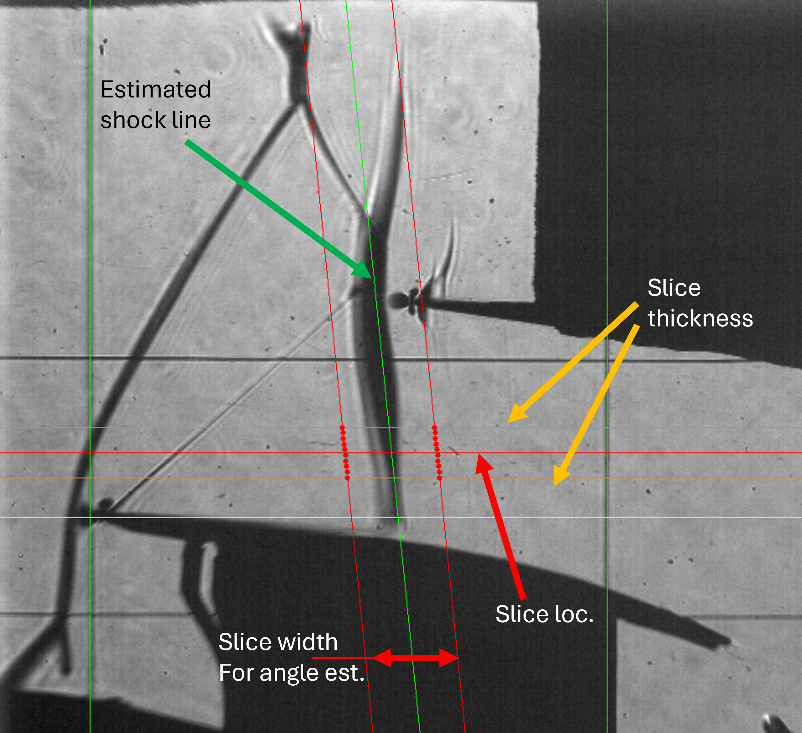
• The inclination_est_info defines the slices width which will be used only to estimate the shock angle and draws the estimated shock line using two points.

• inclination_est_info is list contains [slice_width, firstpoint, secondpoint]

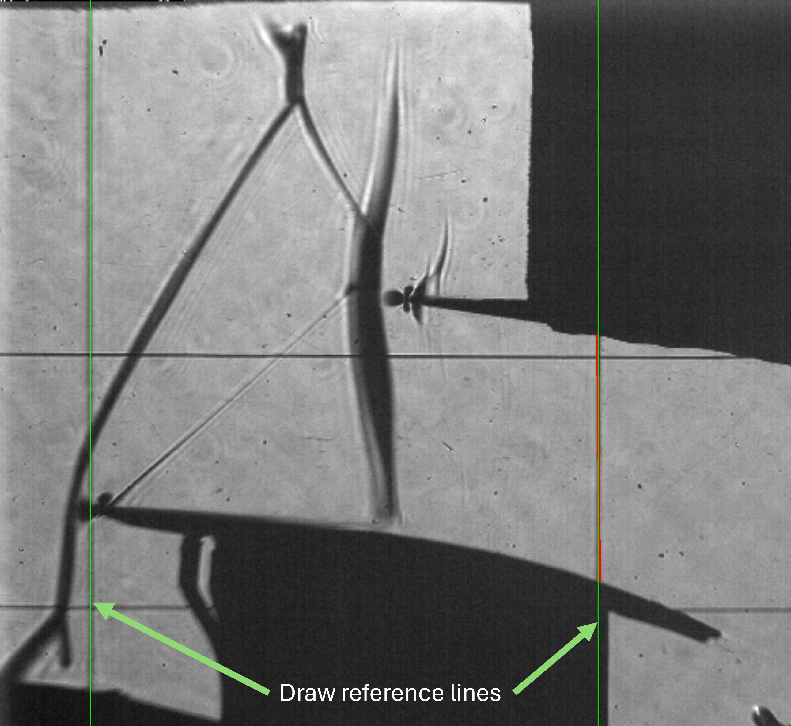
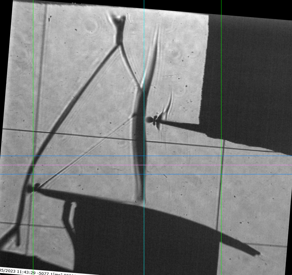
2. Define the scalling lines. Press the left mouse button and drag to draw a line. Two lines will appear: the bold red line represents the start and end mouse locations, and the green line represents the full line. Left-click again to confirm flowed by any keyboard key to close the preview window or right-click to remove the line and try again.

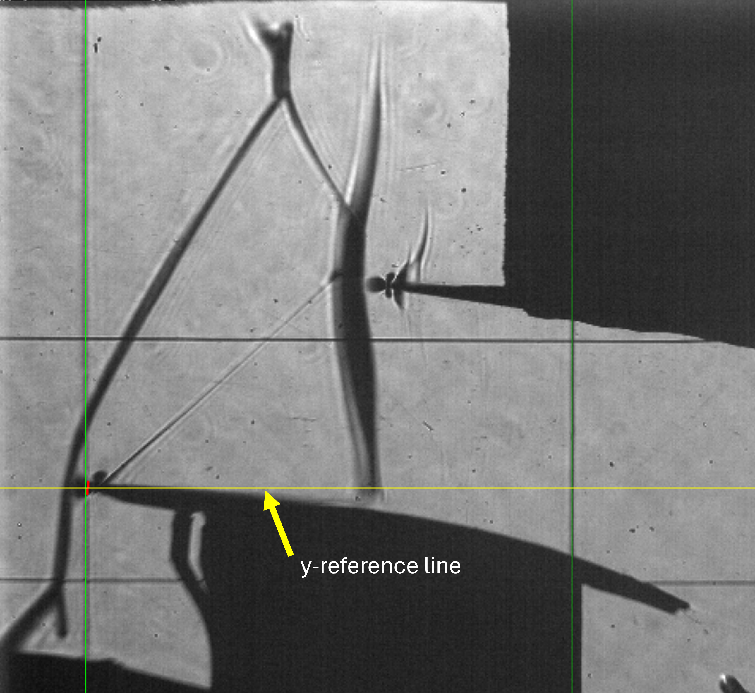
3. Repeat the drawing process to define y-Reference line (the yellow line in this case the leading of the lower profile)

Important

The vertical lines of scaling and the horsintol line of y-reference are defined as the middle point of start and end of the drawn line.

4. The spacified inclination_est_info is reviewed, press any key to continue:

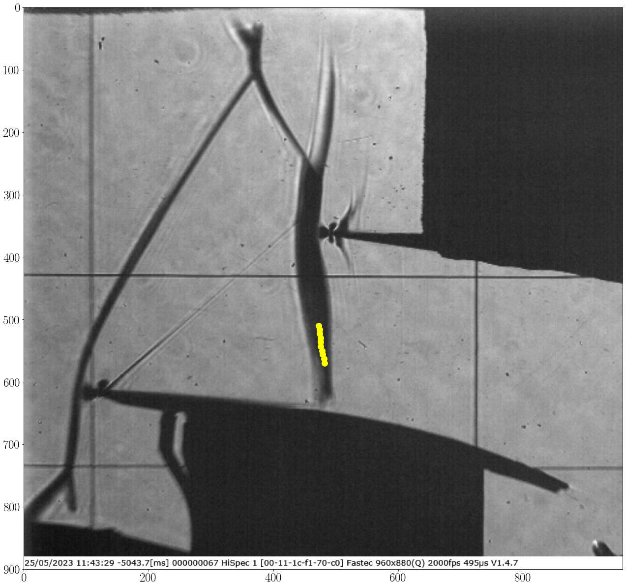
5. The software will estimate the shock angle, store the angle_samples_review and preview the rotated image, press any key to continue:

Img Shape is: (900, 960, 3)
Registered line: 109
Registered line: 726
Image scale: 0.12965964343598055 mm/px
Registered line: 618
Slice center is located at:
   - 541px in absolute reference
   - 9.98mm (77px) from reference `Ref_y0`
Shock angle tracking vertical range above the reference `Ref_y0` is:
   - In (mm)s from 13.87mm to 6.09mm
   - In pixels from 107px to 47px
Shock inclination test and setup ... ✓
Import 33 images for inclination Check ...
[====================] 100%
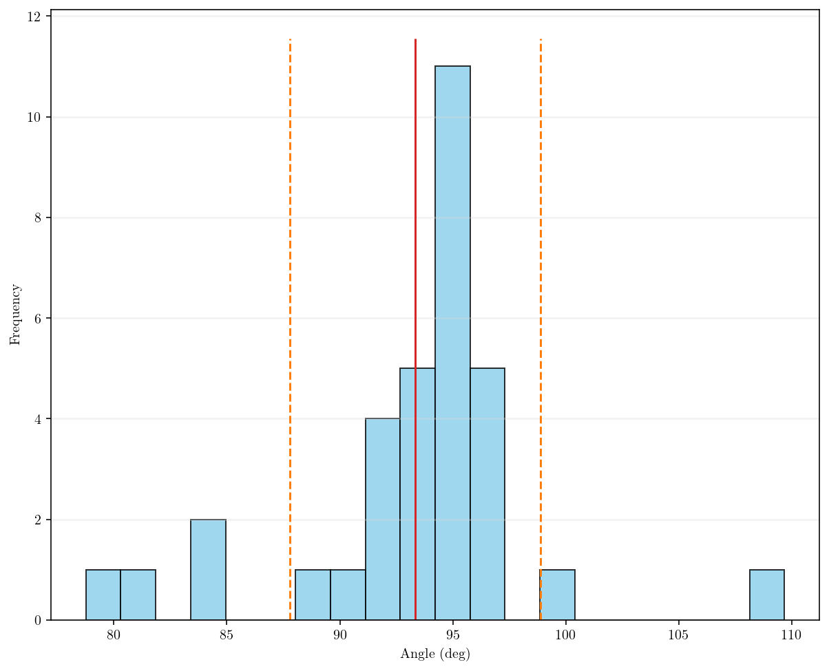
Shock inclination estimation ...
Shock tracking started ... ✓
Angle range variation: [78.77, 109.67],      σ = 5.54
Average shock loc.: 472.20±0.00 px
Average shock angle: 93.34±0.00 deg
Plotting tracked data ...
[====================] 100%
Processing time: 3 Sec

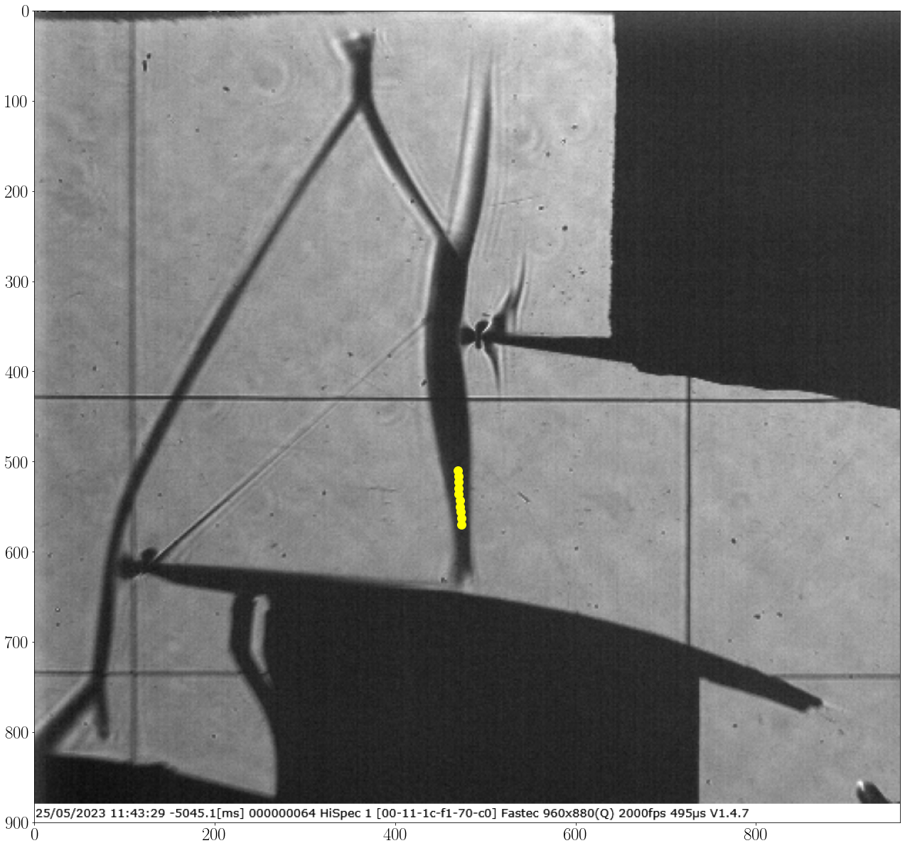
Note

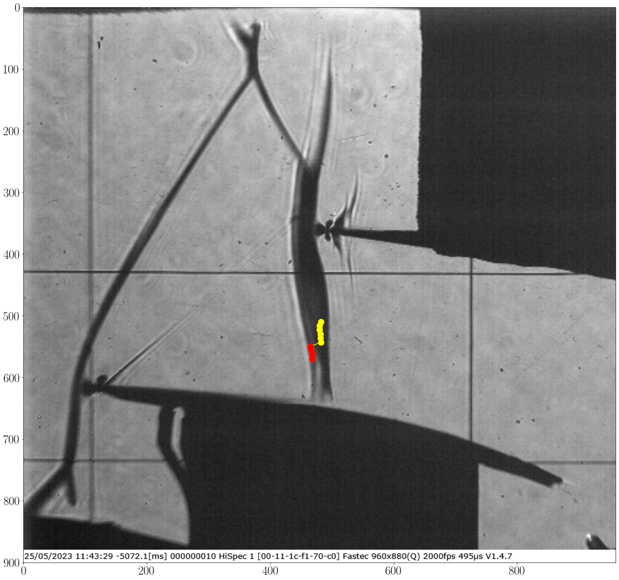
• In the second image, there are red uncertain points that completely miss the location of the Mach wave due to the complexity of the shock shape.

• These uncertain points may affect the overall average angle. It is recommended to use more than 30% of the available data to estimate the shock angle accurately.

• The orange uncertain points do not always indicate a false shock location but suggest the possibility of missing the correct shock location.

• log.txt file is generated at the result location. The log file contain the tracking info. and operations done.

6. The software will generate the slice list and store the data:

RotatedImage: stored ✓
DomainImage: stored ✓
working range is: {'Ref_x0': [109, 726, 618, [(414, 0), (505, 900), 9.909090909090908, -4105.90909090909]], 'Ref_y1': 541, 'avg_shock_angle': array([93.33929034,  0.        ,  0.        ,  0.        ,  5.53565054]), 'avg_shock_loc': array([472.20126383,   0.        ,  13.80257916])}
Importing 100 images ...
[====================] 100%
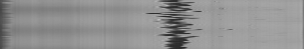
ImageList write: Image list was stored at: results\2.0kHz_10mm_0.12965964343598055mm-px_tk_60px_-SliceList.png

Note

• Working range dicr() can be used to automate the operation later on, very useful for comparing different location of tracking, different slice thickness, etc.

• The slice list is croped by the vertical reference lines to reduce the storage size, the whole width of the iamge can be stored by setting full_img_width = True.

Note

The slice list file name 2.0kHz_10mm_0.12965964343598055mm-px_tk_60px_-SliceList contain all information about the slice according to the provided parameters as follow:

• “2.0kHz” the sampling rate of the images.

• “10mm” is the main slice location.

• “0.12944983818770225mm-px” the scale of each pixels in mm based on D and the drawn vertical reference lines. Also can be defined as the tracking accuracy when the shock is tracked.

• “tk_60px” the defined slice thickness.

• “-SliceList” the comment.

See also

SliceListGenerator.GenerateSlicesArray